Similarity solutions of boundary layer equations for second order fluids

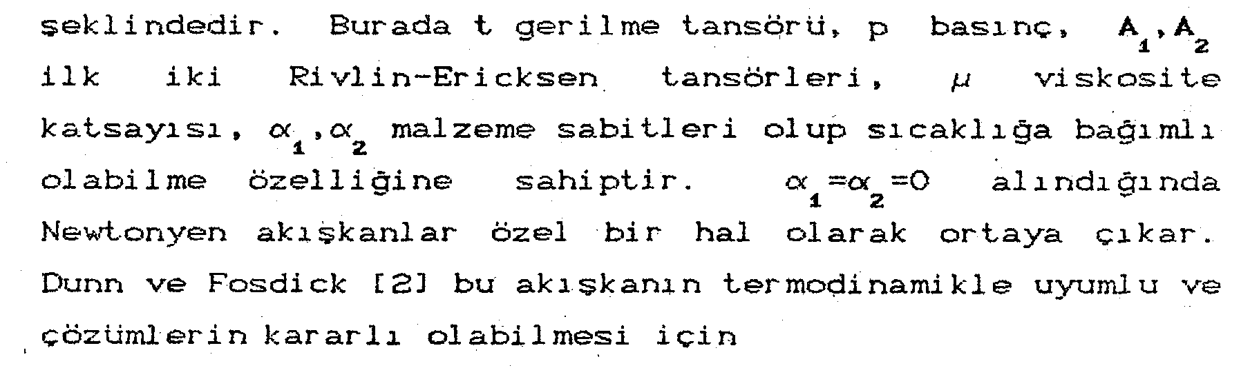
SIMILARITY SOLUTIONS OF BOUNDARY LAYER EQUATIONS FOR SECOND ORDER FLUIDS SUMMARY Navier Stokes theory is adequate to describe the mechanical behaviour of lots of fluids especially those with low molecular weight. The fluids for which the theory is applicable are called Newtonian fluids. For these fluids there is a linear relationship between the stress and velocity gradient. Nonnewtonian fluids are- then described as the fluids for which there is a nonlinear relationship between the stress and velocity gradient of the fluid. Lots of models have been proposed for the constitutive equation of nonnewtonian fluids. One such model which has gained much support from both theorists and experimenters is the second order fluid model. In this model the constitutive equation is given by the following relation t=-pI+^A <-ck A +oc A2 CI > 1 12 2 1 where t is the stress tensor, p pressure, fj viscosity, Ai and A2 are the first two Ri vlin-Ericksen tensors and oa and cxz are the material coefficients which may or may not depend on the temperature. For our study we choose this as a model for an incompressible nonnewtonian fluid. In Chapter 2 taking the starting point as the thermomechanical materials we first derive equation <1 > using the constitutive theory following E123. Then we apply Clausius-Duhem inequality to <1 > to see the restrictions arising from thermodynamics. Following [2] we showed that for <1 > to be compatible with thermodynamics the coefficients should satisty the conditions of +0 <2> 12 ^ In Chapter 3 we first derived the equation of motion of a second order fluid in vectorial notation and then nondi mensi onal i ze the field equations. We then Cv>derived the equation of motion for a special coordinate system. The coordinate system is the network of potential 1 i nes <<£=const. > and streamlines (f -const. ) corresponding to the potential flow around the object. Hence the equations» being an original contribution, arc independent of the body shape immersed into the flow which enables us to solve the equations for an arbitrary body shape. Concentrating our attention to the boundary layer we write an inner and outer expansion corresponding to the inside and outside of the boundary layer- respectively. We then derived the boundary layer equations and boundary conditions which are written w a> r * -^ ? dy> dip a2w^ aw, azw^ aw^, azw^ ± 1 - 1 __£_ +4 Q w 1 -2 Q_ I -Z- I \ <3> ây? d In equation C3> x=0 corresponds to the Navier-Stokes case, the terms in the left of equality are the acceleration terms. Equation <4> is due to incompressibility, W<£ and Wy are the boundary layer velocities in the =W <4>, 0>=0 <5> aw W <>=l, - *<<£,(»>=0 <6> ?'*'?' dy Boundary conditions C5> denote that velocity components are zero at the boundary and <6> are derived by matching the inner and outer expansions. In Chapter 4 we look for the similarity solutions of equation C3> and C4>. Exterior forms are used in finding the solutions. In 4.1 we write the general third order balance equation in exterior form language and then derive the equations leading to the components of isovector fields. In 4.2 we put our boundary layer equations to the form of a balance equation and using the general results of previous section determined the equations for isovector fields. In 4.3 we solved these equations and found all isovector s of the boundary layer equation which are shown below. d <7> <9> The first three vectors correspond to q =const. or flow around a parallel plate. Vi represents a coordinate transformation in dW. dW _ _ ? 4> _ v 3 4> and the velocity components are defined as W,=f <Ç>, W = <13> Substituting <12> and C13> into boundary layer equations C3> and <4> we obtain ordinary differential equations in terms of the similarity variable f2-l+2gf'-Çff '=2f "+« E2gf" '-£ff " ' +2ff ' ' -f,2] <14> Çf'-2g'=0 <15> and the boundary conditions are f<0>=0 g<0>=0 <16> f=0 C17> In the last section of chapter 4 we found V directly by using scaling transformation. Chapter 5 is devoted to the solutions of equations <14> and <15> subject to the conditions <16> and <17>. In the first section we made a series solution near the origin as follows, k a, -1 - 1 f<Ç>=a Ç+f hZ+ a2 Ç4+... C18> ° ' *? 4 J 48 ° 1 f x a -1.. 1 g<ç>= a ç2+ _2_ ç3+ _ a2 Ç*+.... <19> 4 l 12 J 120 The coefficients are in terms of an arbitrary parameter a. Using the series solution by eliminating a between the derivatives of f we can define a relation between the initial conditions «)2-l f = <20> Hence we have reduced the two unknown initial conditions to one. In the following section we look for a numerical solution of equations C14> and <15>. We first reduced the equations into a system of first order differential equations by defininq f =f, f -g, f =f, f fol 1 ows : f =f <21 > 1 3 f ' =çf /'a. <2S> 2 3 f'=f <23> 3 4 f'=</w -2f f +fz>/<2f -Çf > <24> 4 1 13 2 34 143 21 In equation <24> the denominator is zero initially and for f ' to be finite the numerator should be zero which yields exactly the same result as (20 >. The adaptive step size Runge-Kutta method failed to solve the above differential equations so a more specialized initial value method namely Gear method was used to integrate the equations. The one. remainig arbitrary initial condition was determined by shooting. We saw that initial value methods don't work when « >0. 001. So we used finite difference methods to solve the equations for larger x. Due to high nonlinear i ties the initial estimated values should be good to maintain convergence. We use the solutions found from the initial value methods corresponding to x =0. 001 as initial estimates of the finite difference program. The program computed the solutions for various x values. We see that for « >lO0 the program fails to converge for the given boundary conditions. We assumed ini tialy that x was of order 1 so a large value may have no physical interpretation. The solutions for various x values are shown in figures <3-8>. We conclude that increasing x increases the thickness of the boundary layer. In the last section of chapter 5 we outline the general method for finding the profile corresponding to 1/2 the boundary velocity distribution q =oc tp and give a special example for this case namely the stagnation flow. We have to mention that the derivation of the boundary layer equations for the special coordinate system and the solutions are original contributions to the literature. Keyword: Akışkanlar = Fluids ; Hareket denklemleri = Motion equations ; Sınır tabaka denklemleri = Boundary layer equations